Lazy ACF Tiling 

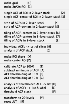
INTRODUCTION

The commands of the Lazy ACF Tiling macro permit

• the calculation and evaluation of single autocorrelation functions (ACFs),
• the calculation and evaluation of strips of ACFs,
• the calculation and evaluation of matrices of ACFs.

Using the Lazy ACF Tiling macro, it is possible to calculate:

• one ACF per image ⇒ bulk ACF: descriptor of bulk size and shape.
• a number of (smaller) ACFs for subregions of the image ⇒ "local" ACFs: descriptors of local size and shape, in other words, descriptors of size and shape variations

• "Local ACFs" can be summed and averaged to yield the bulk ACF of the area.

References:

1. Panozzo Heilbronner, R. (1992). "The autocorrelation function: an image processing tool for fabric analysis." Tectonophysics 212: 351-370.
2. Heilbronner, R. (2002). "Analysis of bulk fabrics and microstructure variations using tilings of autocorrelation functions." Computers & Geosciences 28: 447-455.

    

GETTING STARTED

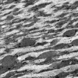
The object of this set of macros is to prepare ACF tilings: a given image is subdivided into a number of squares for which the ACFs (grayvalue images and thresholded versions) are calculated. Using thresholded ACFs, "local" shape analysis is made possible.

• Start Image SXM
• Load Lazy ACF Tiling macro (= text file)
• Open image you wish to analyze
• Prepare two empty images of same size as image
• Combine image windows to stack (= 3 slices)
• Reset measurements in Analyze menu

MAKE GRID

[G] draws grid lines in the desired spacing

Here:
Image size = 256 · 256

Grid spacing = 128

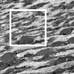
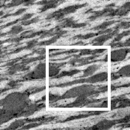
SELECT AREA

[1] creates a square selection box of desired size

(2ⁿ · 2ⁿ, where n = 2, 3, 4 …. etc. = integer number)

Here:
Image size = 256 · 256

Selected size = 128 · 128

Selection box can be moved

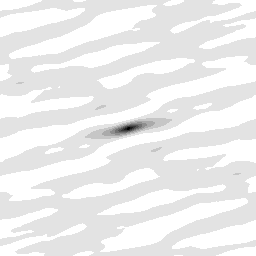
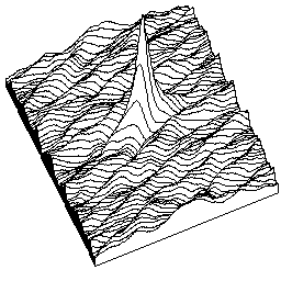
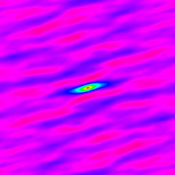
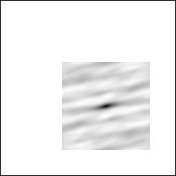
SINGLE ACF

[2] calculates the ACF of the selected area; the ACF is copied into the second slice of the two-layer stack

Here:
Image size = 128 · 128, ACF size = 128 · 128

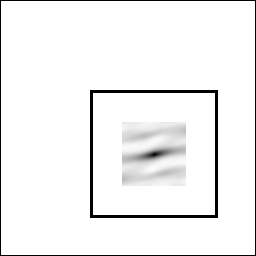
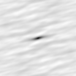
SINGLE ACF CENTER

[3] calculates the ACF of the selected area; the ACF center is copied into the second slice of the two-layer stack

Here:
Image size = 256 · 256, ACF size (= selected) = 128 · 128
⇒ ACF center size = 64 · 64

STRIP OF ACFS

[4] calculates a horizontal strip of ACFs; the ACFs are copied into the second slice of the two-layer stack

Here:
Image size = 256 · 256, ACF size = 64 · 64

The upper left corner = (20,80)
⇒ pixel distance to right hand border = 236
⇒ strip contains 3 ACFs.

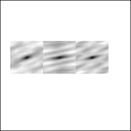
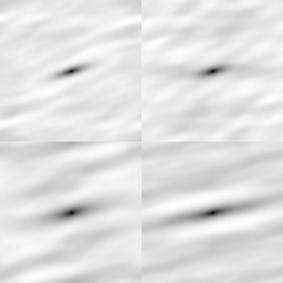
STRIP OF ACF CENTERS

[5] calculates a horizontal strip of ACF centers; the ACF centers are copied into the second slice of the two-layer stack

Here:
The upper left corner = (0,128)
⇒ distance to right hand border = 256 pixel.

Image size = 256 · 256, ACF size = 128 · 128
⇒ ACF center size = 64 · 64. For ACF centers, shift between ACFs = 1/2 ACF size (= ACF center size)
⇒ 3 ACFs (area of last ACF center is shown in black).

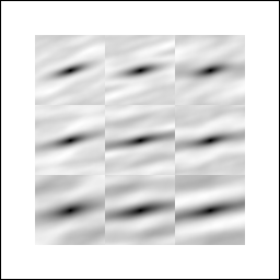
TILING OF ACF CENTERS

[6] calculates a tiling of ACF centers; the ACF centers are copied into the second slice of the TWO-LAYER STACK

Here:
The upper left corner = (0,0)

Image size = 256 · 256, ACF size = 128 · 128 ⇒ ACF center size = 64 · 64. For ACF centers, shift between ACFs = 1/2 ACF size (= ACF center size) ⇒ matrix of 3 · 3 ACFs

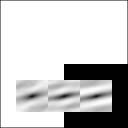
TILING OF ACF CENTERS

[7] calculates a tiling of ACF centers; the ACF centers are copied into the second slice of the THREE-LAYER STACK

Here:
The upper left corner = (0,0)

Image size = 256 · 256, ACF size = 128 · 128
⇒ ACF center size = 64 · 64. For ACF centers, shift between ACFs = 1/2 ACF size (= ACF center size)
⇒ matrix of 3 · 3 ACFs

On the third slice, the ACFs are thresholded.

Here:
The threshold is selected such that the section area = 200 pixels.

TILING OF ACFS

[8] calculates a tiling of ACFs; the thresholded ACF centers are copied into the second slice of the TWO-LAYER STACK

Here:
The upper left corner = (0,0)

Image size = 256 · 256, ACF size = 128 · 128

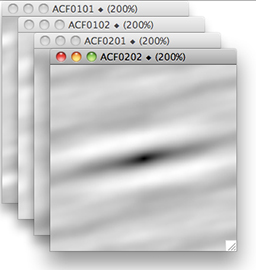
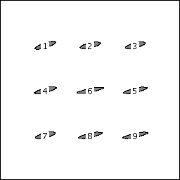
TILING OF ACFS

[9] calculates a set of individual ACFs (corresponding to a tiling of ACFs). The resulting ACFs (slices) are numbered and labeled by rows and columns; they can be combined to ACF stack.

Here:
Image size =256 · 256, ACF size = 128 · 128.
⇒ 2 · 2 ACFs are calculated

ANALYSIS OF ACFS

[0] calculates the bulk ACF from a set of individual ACFs (of equal size).

The ACF stack created by the previous macro ([9]) is thresholded and the thresholded areas are analyzed.

Here:
The threshold is selected such that the section area of the ACF peak = 200 pixels.

DERIVING BULK ACFS

The ACF stack created by the previous macro ([9]) is averaged (sing the SXM Image Stack menu).

For comparison, the ACF of the entire image is also shown. The center parts are the same.

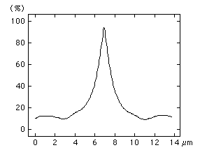
CALIBRATE AND THRESHOLD

[T] is used to calibrate the ACF to 100%.

[A] can be used to set the minimum to 0%,

[B] sets the threshold at 30% (estimated grain size in aggregate),

[C] sets the threshold at 39% (estimated grain size for diluted particles)

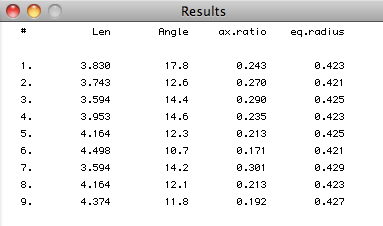
ANALYZE ACFS

[D] calculates perimeter, best fit ellipse (axial ratio and orientation) and equivalent radius of thresholded ACFs.

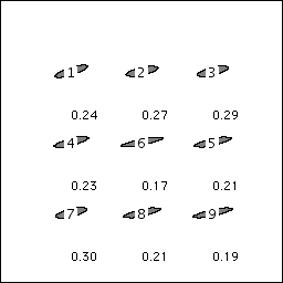
[E] same as [D], adding the results in the image.

[F] performs thresholding of ACFs in stack such that a desired size is obtained.